LearnDS

Clustering - explained

• clustering
• ml
• algorithms

posted on 12 Jun 2020 under category tutorial

Clustering

On supervised learning (e.g. linear regression, decision tree), we already know what we are going to predict (target class, y), such as whether tomorrow will be raining or not. On the contrary, just like its name, unsupervised learning algorithms attempt to find pattern from the data - without knowing the labels (target class, y). One of unsupervised algorithms is clustering.

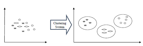
So, Clustering is the task of grouping data into two or more groups based on the properties of the data, and more exactly based on certain patterns which are more or less obvious in the data. The goal is to find those patterns in the data that help us be sure that, given a certain item in our dataset, we will be able to correctly place the item in a correct group, so that it is similar to other items in that group, but different from items in other groups. That means the clustering actually consists of two parts: one is to identify the groups and the other one is to try as much as possible to place every item in the correct group.

The ideal result for a clustering algorithm is that two items in the same group are as similar to each other, while two items from different groups are as different as possible.

It can be used for various things:

• ✔ Customer segmentation for the purpose of marketing.
• ✔ Customer purchasing behavior analysis for promotions and discounts.
• ✔ Identifying geo-clusters in an epidemic outbreak such as COVID-19.

A real-world brief example would be customer segmentation. As a business selling various type of products, it would be very difficult to find the perfect business strategy for each and every customer. But we can be smart about it and try to group our customers into a few subgroups, understand what those customers all have in common and adapt our business strategy for every group. Coming up with the wrong business strategy to a customer would mean perhaps losing that customer, so it’s important that we’ve achieved a good clustering of our market.

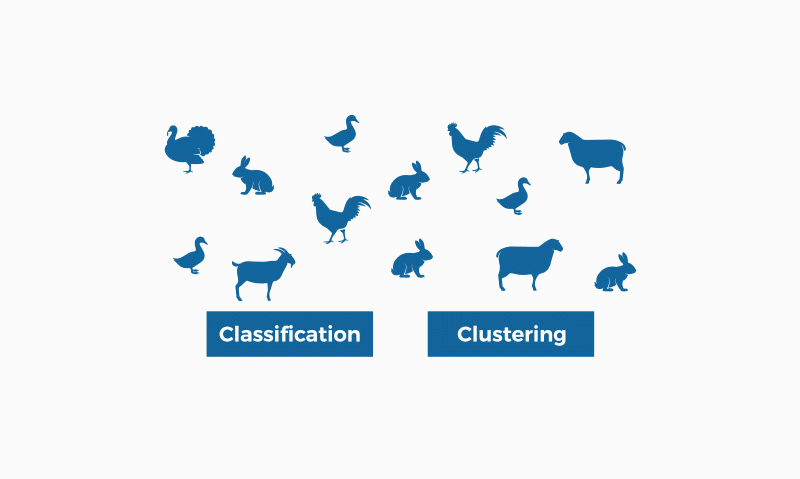
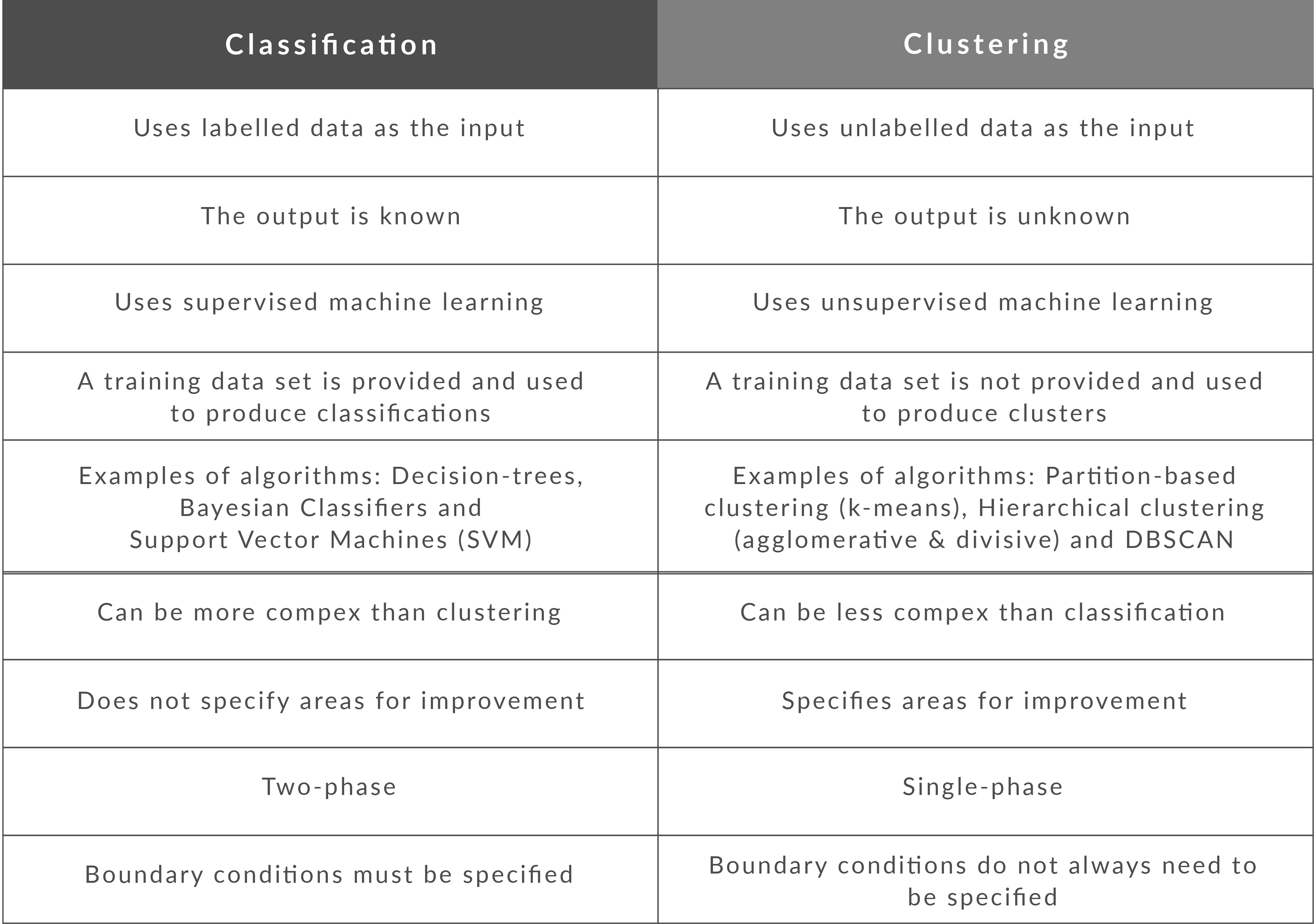
What is the difference between Clustering and Classification

Classification is the result of supervised learning which means that there is a known label that you want the system to generate. For example, if you built a fruit classifier, it would say “this is an orange, this is an apple”, based on you showing it examples of apples and oranges.

Clustering is the result of unsupervised learning which means that you’ve seen lots of examples, but don’t have labels. In this case, the clustering might return with “fruits with soft skin and lots of dimples”, “fruits with shiny hard skin” and “elongated yellow fruits” based not merely showing lots of fruit to the system, but not identifying the names of different types of fruit. Moreover, they are called clusters

Types of Clustering

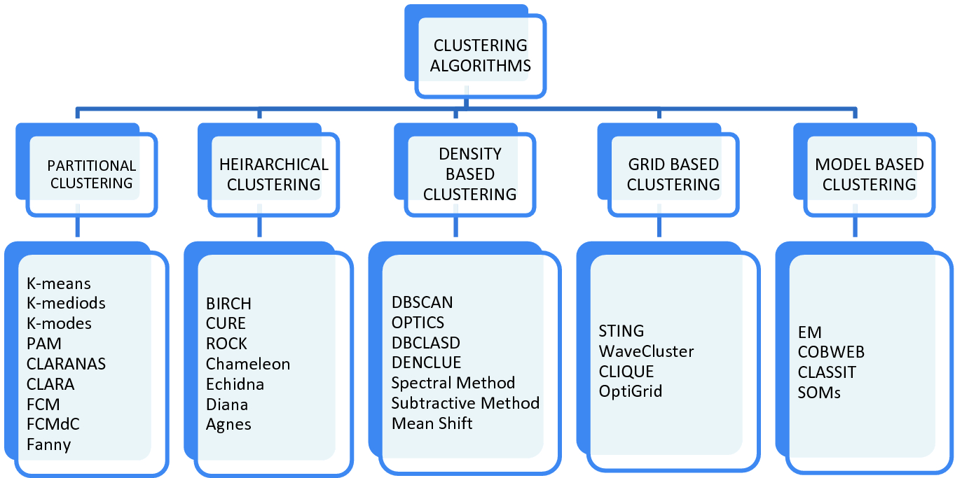
Given the subjective nature of clustering tasks, there are various algorithms that suit different types of problems. Each algorithm has its own rules and the mathematics behind how clusters are calculated. Clustering can be of many types based on Cluster Formation Methods. Followings are some other cluster formation methods −

Density-based

In these methods, the clusters are formed as the dense region. The advantage of these methods is that they have good accuracy as well as good ability to merge two clusters. Ex. Density-Based Spatial Clustering of Applications with Noise (DBSCAN), Ordering Points to identify Clustering structure (OPTICS) etc.

Hierarchical-based

In these methods, the clusters are formed as a tree type structure based on the hierarchy. They have two categories namely, Agglomerative (Bottom up approach) and Divisive (Top down approach). Ex. Clustering using Representatives (CURE), Balanced iterative Reducing Clustering using Hierarchies (BIRCH) etc.

Partitioning

In these methods, the clusters are formed by portioning the objects into k clusters. Number of clusters will be equal to the number of partitions. Ex. K-means, K-mediodes, PAM, Clustering Large Applications based upon randomized Search (CLARANS) etc.

Grid

In these methods, the clusters are formed as a grid like structure. The advantage of these methods is that all the clustering operation done on these grids are fast and independent of the number of data objects. Ex. Statistical Information Grid (STING), Clustering in Quest (CLIQUE).

A broad Classification of types of Clustering Algorithms is given below.

Clustering Performance Evaluation

There are various functions with the help of which we can evaluate the performance of clustering algorithms. Following are some important and mostly used functions for evaluating clustering performance −

Adjusted Rand Index

Rand Index is a function that computes a similarity measure between two clustering. For this computation rand index considers all pairs of samples and counting pairs that are assigned in the similar or different clusters in the predicted and true clustering. Afterwards, the raw Rand Index score is ‘adjusted for chance’ into the Adjusted Rand Index score by using the following formula −

AdjustedRI=(RI−Expected−RI)/(max(RI)−Expected−RI)

Perfect labeling would be scored 1 and bad labelling or independent labelling is scored 0 or negative.

Mutual Information Based Score

Mutual Information computes the agreement of the two assignments. It ignores the permutations. The Mutual Information score expresses the extent to which observed frequency of co-occurrence differs from what we would expect (statistically speaking). In statistically pure terms this is a measure of the strength of association between words x and y. There are following versions available −

Normalized Mutual Information (NMI)

Normalized Mutual Information (NMI) is a normalization of the Mutual Information (MI) score to scale the results between 0 (no mutual information) and 1 (perfect correlation). In this function, mutual information is normalized by some generalized mean of H(labels_true) and H(labels_pred)), defined by the average_method.

Adjusted Mutual Information (AMI)

Adjusted Mutual Information (AMI) is an adjustment of the Mutual Information (MI) score to account for chance. It accounts for the fact that the MI is generally higher for two clusterings with a larger number of clusters, regardless of whether there is actually more information shared.

Fowlkes-Mallows Score

The Fowlkes-Mallows function measures the similarity of two clustering of a set of points. It may be defined as the geometric mean of the pairwise precision and recall.

Mathematically,

FMS=TP/√(TP+FP)(TP+FN)

Here, TP = True Positive − number of pair of points belonging to the same clusters in true as well as predicted labels both.

FP = False Positive − number of pair of points belonging to the same clusters in true labels but not in the predicted labels.

FN = False Negative − number of pair of points belonging to the same clusters in the predicted labels but not in the true labels.

Silhouette Coefficient

The Silhouette function will compute the mean Silhouette Coefficient of all samples using the mean intra-cluster distance and the mean nearest-cluster distance for each sample.

Mathematically,

S=(b−a)/max(a,b) Here, a is intra-cluster distance.

and, b is mean nearest-cluster distance.

Contingency Matrix

This matrix will report the intersection cardinality for every trusted pair of (true, predicted). Confusion matrix for classification problems is a square contingency matrix.

Comparing Python Clustering Algorithms

There are a lot of clustering algorithms to choose from. The standard sklearn clustering suite has thirteen different clustering classes alone. So what clustering algorithms should you be using? As with every question in data science and machine learning it depends on your data. A number of those thirteen classes in sklearn are specialised for certain tasks (such as co-clustering and bi-clustering, or clustering features instead data points). Obviously an algorithm specializing in text clustering is going to be the right choice for clustering text data, and other algorithms specialize in other specific kinds of data. Thus, if you know enough about your data, you can narrow down on the clustering algorithm that best suits that kind of data, or the sorts of important properties your data has, or the sorts of clustering you need done.

K-Means

K-Means is the ‘go-to’ clustering algorithm for many simply because it is fast, easy to understand, and available everywhere (there’s an implementation in almost any statistical or machine learning tool you care to use). K-Means has a few problems however. The first is that it isn’t a clustering algorithm, it is a partitioning algorithm. That is to say K-means doesn’t ‘find clusters’ it partitions your dataset into as many (assumed to be globular) chunks as you ask for by attempting to minimize intra-partition distances. That leads to the second problem: you need to specify exactly how many clusters you expect. If you know a lot about your data then that is something you might expect to know. If, on the other hand, you are simply exploring a new dataset then ‘number of clusters’ is a hard parameter to have any good intuition for. The usually proposed solution is to run K-Means for many different ‘number of clusters’ values and score each clustering with some ‘cluster goodness’ measure (usually a variation on intra-cluster vs inter-cluster distances) and attempt to find an ‘elbow’. If you’ve ever done this in practice you know that finding said elbow is usually not so easy, nor does it necessarily correlate as well with the actual ‘natural’ number of clusters as you might like. Finally K-Means is also dependent upon initialization; give it multiple different random starts and you can get multiple different clusterings. This does not engender much confidence in any individual clustering that may result.

So, in summary, here’s how K-Means seems to stack up against out desiderata:

• Don’t be wrong!: K-means is going to throw points into clusters whether they belong or not; it also assumes you clusters are globular. K-Means scores very poorly on this point.
• Intuitive parameters: If you have a good intuition for how many clusters the dataset your exploring has then great, otherwise you might have a problem.
• Stability: Hopefully the clustering is stable for your data. Best to have many runs and check though.
• Performance: This is K-Means big win. It’s a simple algorithm and with the right tricks and optimizations can be made exceptionally efficient. There are few algorithms that can compete with K-Means for performance. If you have truly huge data then K-Means might be your only option.

Affinity Propagation

Affinity Propagation is a newer clustering algorithm that uses a graph based approach to let points ‘vote’ on their preferred ‘exemplar’. The end result is a set of cluster ‘exemplars’ from which we derive clusters by essentially doing what K-Means does and assigning each point to the cluster of it’s nearest exemplar. Affinity Propagation has some advantages over K-Means. First of all the graph based exemplar voting means that the user doesn’t need to specify the number of clusters. Second, due to how the algorithm works under the hood with the graph representation it allows for non-metric dissimilarities (i.e. we can have dissimilarities that don’t obey the triangle inequality, or aren’t symmetric). This second point is important if you are ever working with data isn’t naturally embedded in a metric space of some kind; few clustering algorithms support, for example, non-symmetric dissimilarities. Finally Affinity Propagation does, at least, have better stability over runs (but not over parameter ranges!).

The weak points of Affinity Propagation are similar to K-Means. Since it partitions the data just like K-Means we expect to see the same sorts of problems, particularly with noisy data. While Affinity Propagation eliminates the need to specify the number of clusters, it has ‘preference’ and ‘damping’ parameters. Picking these parameters well can be difficult. The implementation in sklearn default preference to the median dissimilarity. This tends to result in a very large number of clusters. A better value is something smaller (or negative) but data dependent. Finally Affinity Propagation is slow; since it supports non-metric dissimilarities it can’t take any of the shortcuts available to other algorithms, and the basic operations are expensive as data size grows.

So, in summary, over our desiderata we have:

• Don’t be wrong: The same issues as K-Means; Affinity Propagation is going to throw points into clusters whether they belong or not; it also assumes you clusters are globular.
• Intuitive Parameters: It can be easier to guess at preference and damping than number of clusters, but since Affinity Propagation is quite sensitive to preference values it can be fiddly to get “right”. This isn’t really that much of an improvement over K-Means.
• Stability: Affinity Propagation is deterministic over runs.
• Performance: Affinity Propagation tends to be very slow. In practice running it on large datasets is essentially impossible without a carefully crafted and optimized implementation (i.e. not the default one available in sklearn).

Mean Shift

Mean shift is another option if you don’t want to have to specify the number of clusters. It is centroid based, like K-Means and affinity propagation, but can return clusters instead of a partition. The underlying idea of the Mean Shift algorithm is that there exists some probability density function from which the data is drawn, and tries to place centroids of clusters at the maxima of that density function. It approximates this via kernel density estimation techniques, and the key parameter is then the bandwidth of the kernel used. This is easier to guess than the number of clusters, but may require some staring at, say, the distributions of pairwise distances between data points to choose successfully. The other issue (at least with the sklearn implementation) is that it is fairly slow depsite potentially having good scaling!

How does Mean Shift fare against out criteria? In principle proming, but in practice …

• Don’t be wrong!: Mean Shift doesn’t cluster every point, but it still aims for globular clusters, and in practice it can return less than ideal results (see below for example). Without visual validation it can be hard to know how wrong it may be.
• Intuitive parameters: Mean Shift has more intuitive and meaningful parameters; this is certainly a strength.
• Stability: Mean Shift results can vary a lot as you vary the bandwidth parameter (which can make selection more difficult than it first appears. It also has a random initialisation, which means stability under runs can vary (if you reseed the random start).
• Performance: While Mean Shift has good scalability in principle (using ball trees) in practice the sklearn implementation is slow; this is a serious weak point for Mean Shift.

Spectral Clustering

Spectral clustering can best be thought of as a graph clustering. For spatial data one can think of inducing a graph based on the distances between points (potentially a k-NN graph, or even a dense graph). From there spectral clustering will look at the eigenvectors of the Laplacian of the graph to attempt to find a good (low dimensional) embedding of the graph into Euclidean space. This is essentially a kind of manifold learning, finding a transformation of our original space so as to better represent manifold distances for some manifold that the data is assumed to lie on. Once we have the transformed space a standard clustering algorithm is run; with sklearn the default is K-Means. That means that the key for spectral clustering is the transformation of the space. Presuming we can better respect the manifold we’ll get a better clustering – we need worry less about K-Means globular clusters as they are merely globular on the transformed space and not the original space. We unfortunately retain some of K-Means weaknesses: we still partition the data instead of clustering it; we have the hard to guess ‘number of clusters’ parameter; we have stability issues inherited from K-Means. Worse, if we operate on the dense graph of the distance matrix we have a very expensive initial step and sacrifice performance.

So, in summary:

• Don’t be wrong!: We are less wrong, in that we don’t have a purely globular cluster assumption; we do still have partitioning and hence are polluting clusters with noise, messing with our understanding of the clusters and hence the data.
• Intuitive parameters: We are no better than K-Means here; we have to know the correct number of clusters, or hope to guess by clustering over a range of parameter values and finding some way to pick the ‘right one’.
• Stability: Slightly more stable than K-Means due to the transformation, but we still suffer from those issues.
• Performance: For spatial data we don’t have a sparse graph (unless we prep one ourselves) so the result is a somewhat slower algorithm.

Agglomerative Clustering

Agglomerative clustering is really a suite of algorithms all based on the same idea. The fundamental idea is that you start with each point in it’s own cluster and then, for each cluster, use some criterion to choose another cluster to merge with. Do this repeatedly until you have only one cluster and you get get a hierarchy, or binary tree, of clusters branching down to the last layer which has a leaf for each point in the dataset. The most basic version of this, single linkage, chooses the closest cluster to merge, and hence the tree can be ranked by distance as to when clusters merged/split. More complex variations use things like mean distance between clusters, or distance between cluster centroids etc. to determine which cluster to merge. Once you have a cluster hierarchy you can choose a level or cut (according to some criteria) and take the clusters at that level of the tree. For sklearn we usually choose a cut based on a ‘number of clusters’ parameter passed in.

The advantage of this approach is that clusters can grow ‘following the underlying manifold’ rather than being presumed to be globular. You can also inspect the dendrogram of clusters and get more information about how clusters break down. On the other hand, if you want a flat set of clusters you need to choose a cut of the dendrogram, and that can be hard to determine. You can take the sklearn approach and specify a number of clusters, but as we’ve already discussed that isn’t a particularly intuitive parameter when you’re doing EDA. You can look at the dendrogram and try to pick a natural cut, but this is similar to finding the ‘elbow’ across varying k values for K-Means: in principle it’s fine, and the textbook examples always make it look easy, but in practice on messy real world data the ‘obvious’ choice is often far from obvious. We are also still partitioning rather than clustering the data, so we still have that persistent issue of noise polluting our clusters. Fortunately performance can be pretty good; the sklearn implementation is fairly slow, but fastcluster <https://pypi.python.org/pypi/fastcluster>__ provides high performance agglomerative clustering if that’s what you need.

So, in summary:

• Don’t be wrong!: We have gotten rid of the globular assumption, but we are still assuming that all the data belongs in clusters with no noise.
• Intuitive parameters: Similar to K-Means we are stuck choosing the number of clusters (not easy in EDA), or trying to discern some natural parameter value from a plot that may or may not have any obvious natural choices.
• Stability: Agglomerative clustering is stable across runs and the dendrogram shows how it varies over parameter choices (in a reasonably stable way), so stability is a strong point.
• Performance: Performance can be good if you get the right implementation.

DBSCAN

DBSCAN is a density based algorithm – it assumes clusters for dense regions. It is also the first actual clustering algorithm we’ve looked at: it doesn’t require that every point be assigned to a cluster and hence doesn’t partition the data, but instead extracts the ‘dense’ clusters and leaves sparse background classified as ‘noise’. In practice DBSCAN is related to agglomerative clustering. As a first step DBSCAN transforms the space according to the density of the data: points in dense regions are left alone, while points in sparse regions are moved further away. Applying single linkage clustering to the transformed space results in a dendrogram, which we cut according to a distance parameter (called epsilon or eps in many implementations) to get clusters. Importantly any singleton clusters at that cut level are deemed to be ‘noise’ and left unclustered. This provides several advantages: we get the manifold following behaviour of agglomerative clustering, and we get actual clustering as opposed to partitioning. Better yet, since we can frame the algorithm in terms of local region queries we can use various tricks such as kdtrees to get exceptionally good performance and scale to dataset sizes that are otherwise unapproachable with algorithms other than K-Means. There are some catches however. Obviously epsilon can be hard to pick; you can do some data analysis and get a good guess, but the algorithm can be quite sensitive to the choice of the parameter. The density based transformation depends on another parameter (min_samples in sklearn). Finally the combination of min_samples and eps amounts to a choice of density and the clustering only finds clusters at or above that density; if your data has variable density clusters then DBSCAN is either going to miss them, split them up, or lump some of them together depending on your parameter choices.

So, in summary:

• Don’t be wrong!: Clusters don’t need to be globular, and won’t have noise lumped in; varying density clusters may cause problems, but that is more in the form of insufficient detail rather than explicitly wrong. DBSCAN is the first clustering algorithm we’ve looked at that actually meets the ‘Don’t be wrong!’ requirement.
• Intuitive parameters: Epsilon is a distance value, so you can survey the distribution of distances in your dataset to attempt to get an idea of where it should lie. In practice, however, this isn’t an especially intuitive parameter, nor is it easy to get right.
• Stability: DBSCAN is stable across runs (and to some extent subsampling if you re-parameterize well); stability over varying epsilon and min samples is not so good.
• Performance: This is DBSCAN’s other great strength; few clustering algorithms can tackle datasets as large as DBSCAN can.

In next blogs, we will discuss the various algorithms related to Clustering Analysis.

---

Want to support this project? Contribute..