Regression - explained

• ml
• regression
• algorithms

posted on 09 Jun 2020 under category tutorial

Regression

What is Regression?

Regression analysis is a statistical method to model the relationship between a dependent (target) variable and independent (predictor) variables with one or more independent variables. More specifically, Regression analysis helps us to understand how the value of the dependent variable is changing corresponding to an independent variable when other independent variables are held fixed. It predicts continuous/real values such as temperature, age, salary, price, etc.

We can understand the concept of regression analysis using the below example:

Example: Suppose there is a marketing company A, who does various advertisement every year and get sales on that. The below list shows the advertisement made by the company in the last 5 years and the corresponding sales:

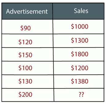
Now, the company wants to do the advertisement of $200 in the year 2019 and wants to know the prediction about the sales for this year. So to solve such type of prediction problems in machine learning, we need regression analysis.

Regression is a supervised learning technique which helps in finding the correlation between variables and enables us to predict the continuous output variable based on the one or more predictor variables. It is mainly used for prediction, forecasting, time series modeling, and determining the causal-effect relationship between variables.

In Regression, we plot a graph between the variables which best fits the given datapoints, using this plot, the machine learning model can make predictions about the data. In simple words, “Regression shows a line or curve that passes through all the datapoints on target-predictor graph in such a way that the vertical distance between the datapoints and the regression line is minimum.” The distance between datapoints and line tells whether a model has captured a strong relationship or not.

Some examples of regression can be as:

• Prediction of rain using temperature and other factors
• Determining Market trends
• Prediction of road accidents due to rash driving.

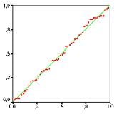
We can observe that the given plot represents a somehow linear relationship between the mileage and displacement of cars. The green points are the actual observations while the black line fitted is the line of regression

Linear Regression

Linear regression is a technique used to analyze a linear relationship between input variables and a single output variable. A linear relationship means that the data points tend to follow a straight line. Simple linear regression involves only a single input variable. Figure 1 shows a data set with a linear relationship.

The idea is to fit a straight line in the n-dimensional space that holds all our observational points. This would constitute forming an equation of the form y = mx + c. Because we have multiple variables, we might need to extend this mx to be m₁x₁, m₂x₂ and so on. This extensions results in the following mathematical representation between the independent and dependent variables:

where

1. y = dependent variable/outcome
2. x₁ to x_n are the dependent variables
3. b₀ to b_n are the coefficients of the linear model

A linear regression models bases itself on the following assumptions:

1. Linearity
2. Homoscedasticity or
3. Multivariate Normality
4. Independence of errors
5. Lack of multicollinearity

If these assumptions do not hold, then linear regression probably isn’t the model for your problem.

When to Use Linear Regression

Linear regression is a useful technique but isn’t always the right choice for your data. Linear regression is a good choice when there is a linear relationship between your independent and dependent variables and you are trying to predict continuous values.

It is not a good choice when the relationship between independent and dependent variables is more complicated or when outputs are discrete values.

Assumptions of Linear Regression

• A note about sample size. In Linear regression the sample size rule of thumb is that the regression analysis requires at least 20 cases per independent variable in the analysis.

The regression has five key assumptions:

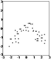
• Linear relationship First, linear regression needs the relationship between the independent and dependent variables to be linear. It is also important to check for outliers since linear regression is sensitive to outlier effects. The linearity assumption can best be tested with scatter plots, the following two examples depict two cases, where no and little linearity is present.

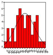
• Multivariate normality Secondly, the linear regression analysis requires all variables to be multivariate normal. This assumption can best be checked with a histogram or a Q-Q-Plot. Normality can be checked with a goodness of fit test, e.g., the Kolmogorov-Smirnov test. When the data is not normally distributed a non-linear transformation (e.g., log-transformation) might fix this issue.

• No or little multicollinearity Thirdly, linear regression assumes that there is little or no multicollinearity in the data. Multicollinearity occurs when the independent variables are too highly correlated with each other. Multicollinearity may be tested with three central criteria:

1) Correlation matrix – when computing the matrix of Pearson’s Bivariate Correlation among all independent variables the correlation coefficients need to be smaller than 1. 2) Tolerance – the tolerance measures the influence of one independent variable on all other independent variables; the tolerance is calculated with an initial linear regression analysis. Tolerance is defined as T = 1 – R² for these first step regression analysis. With T < 0.1 there might be multicollinearity in the data and with T < 0.01 there certainly is. 3) Variance Inflation Factor (VIF) – the variance inflation factor of the linear regression is defined as VIF = 1/T. With VIF > 5 there is an indication that multicollinearity may be present; with VIF > 10 there is certainly multicollinearity among the variables.

If multicollinearity is found in the data, centering the data (that is deducting the mean of the variable from each score) might help to solve the problem. However, the simplest way to address the problem is to remove independent variables with high VIF values.

4) Condition Index – the condition index is calculated using a factor analysis on the independent variables. Values of 10-30 indicate a mediocre multicollinearity in the linear regression variables, values > 30 indicate strong multicollinearity.

If multicollinearity is found in the data centering the data, that is deducting the mean score might help to solve the problem. Other alternatives to tackle the problems is conducting a factor analysis and rotating the factors to insure independence of the factors in the linear regression analysis.

• No auto-correlation Fourthly, linear regression analysis requires that there is little or no autocorrelation in the data. Autocorrelation occurs when the residuals are not independent from each other. In other words when the value of y(x+1) is not independent from the value of y(x).

While a scatterplot allows you to check for autocorrelations, you can test the linear regression model for autocorrelation with the Durbin-Watson test. Durbin-Watson’s d tests the null hypothesis that the residuals are not linearly auto-correlated. While d can assume values between 0 and 4, values around 2 indicate no autocorrelation. As a rule of thumb values of 1.5 < d < 2.5 show that there is no auto-correlation in the data. However, the Durbin-Watson test only analyses linear autocorrelation and only between direct neighbors, which are first order effects.

• Homoscedasticity

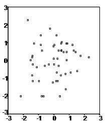
The last assumption of the linear regression analysis is homoscedasticity. The scatter plot is good way to check whether the data are homoscedastic (meaning the residuals are equal across the regression line). The following scatter plots show examples of data that are not homoscedastic (i.e., heteroscedastic):

The Goldfeld-Quandt Test can also be used to test for heteroscedasticity. The test splits the data into two groups and tests to see if the variances of the residuals are similar across the groups. If homoscedasticity is present, a non-linear correction might fix the problem.

Above, we discussed what is Regression and the assumptions or so called limitations of linear regression. Linear Regression is assumed to be the simplest machine learning algorithm the world has ever seen, and yes! it is! We also discussed how your model can give you poor predictions in real time if you don’t obey the assumptions of linear regression. Whatever you are going to predict, whether it is stock value, sales or some revenue, linear regression must be handled with care if you want to get best values from it.

Multiple Linear Regression

When you have only 1 independent variable and 1 dependent variable, it is called simple linear regression. When you have more than 1 independent variable and 1 dependent variable, it is called Multiple linear regression.

so, when there are more than one independent variable (x1,x2,x3…xn) and one dependent variable (y), its called Multiple Linear Regression. Most linear Regressions are multiple linear regression itself.

Here ‘y’ is the dependent variable to be estimated, and X are the independent variables and ε is the error term. βi’s are the regression coefficients.

Polynomial Linear Regression

This regression allows us to regress over dependent variable(s) that has a polynomial relationship with the independent variables generally represented.

Non Linear Regression

As we saw, linear regression says, the data should be linear in nature, there must be a linear relationship. But, wait! the real world data is always non-linear. Yes, so, what should we do, should we try to bring non-linearity into the regression model, or check out the residuals and fitted values, or keep applying transformations and working harder and harder to get the best predictive model using linear regression. Yes or No? Now, the question is.. is there any other way to deal with this, so that we can get a better predictive model without getting into these assumptions of linear regression.

Yes! there is a solution, in fact a bunch of solutions.

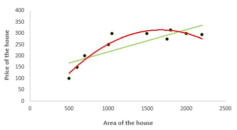
Polynomial Regression

It is a technique to fit a nonlinear equation by taking polynomial functions of independent variable. In the figure given below, you can see the red curve fits the data better than the green curve. Hence in the situations where the relation between the dependent and independent variable seems to be non-linear we can deploy Polynomial Regression Models.

Thus a polynomial of degree k in one variable is written as:

Here we can create new features like

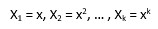
and can fit linear regression in the similar manner.

In case of multiple variables say X1 and X2, we can create a third new feature (say X3) which is the product of X1 and X2 i.e.

Disclaimer: It is to be kept in mind that creating unnecessary extra features or fitting polynomials of higher degree may lead to overfitting.

Quantile Regression

Quantile regression is the extension of linear regression and we generally use it when outliers, high skeweness and heteroscedasticity exist in the data.

In linear regression, we predict the mean of the dependent variable for given independent variables. Since mean does not describe the whole distribution, so modeling the mean is not a full description of a relationship between dependent and independent variables. So we can use quantile regression which predicts a quantile (or percentile) for given independent variables. The term “quantile” is the same as “percentile”

Advantages of Quantile over Linear Regression

• Quite beneficial when heteroscedasticity is present in the data.
• Robust to outliers
• Distribution of dependent variable can be described via various quantiles.
• It is more useful than linear regression when the data is skewed.

Generalised Regression Model

There are many different analytic procedures for fitting regressive models of nonlinear nature (e.g., Generalized Linear/Nonlinear Models (GLZ), Generalized Additive Models (GAM), etc.), or more better models called tree based regressive models, boosted tree based based, support vector machine based regression model etc.

Most of us know about Decision Trees and Random Forest, it is very common, in case of classification or regression and it is also true that they often perform far better than other regression models with minimum efforts. So, now we will be talking about tree based models such as Decision Trees and ensemble tree based like Random forests. Tree based model have proven themselves to be both reliable and effective, and are now part of any modern predictive modeler’s toolkit.

The bottom line is: You can spend 3 hours playing with the data, generating features and interaction variables for linear regression and get a 77% r-squared; and I can “from sklearn.ensemble import RandomForestRegressor” and in 3 minutes get an 82% r-squared. I am not creating a hype for these tree model, but its the truth.

Let me explain it using some examples for clear intuition with an example. Linear regression is a linear model, which means it works really nicely when the data has a linear shape. But, when the data has a non-linear shape, then a linear model cannot capture the non-linear features. So in this case, you can use the decision trees, which do a better job at capturing the non-linearity in the data by dividing the space into smaller sub-spaces depending on the rules that exist.

Now, the question is when do you use linear regression vs Trees? Let’s suppose you are trying to predict income. The predictor variables that are available are education, age, and city. Now in a linear regression model, you have an equation with these three attributes. Fine. You’d expect higher degrees of education, higher “age” and larger cities to be associated with higher income. But what about a PhD who is 40 years old and living in Scranton Pennsylvania? Is he likely to earn more than a BS holder who is 35 and living in Upper West SIde NYC? Maybe not. Maybe education totally loses its predictive power in a city like Scranton? Maybe age is a very ineffective, weak variable in a city like NYC?

Tree based Regression

This is where decision trees are handy. The tree can split by city and you get to use a different set of variables for each city. Maybe Age will be a strong second-level split variable in Scranton, but it might not feature at all in the NYC branch of the tree. Education may be a stronger variable in NYC.

Decision Trees, be it Random Forest or Gradient Bossted Machine based Regression, handle messier data and messier relationships better than regression models. ANd there is seldom a dataset in the real world where relationships are not messy. No wonder you will seldom see a linear regression model outperforming RF or GBM. So, this is the main idea behind tree (Decision Tree Regression) and ensemble based models (Random Forest Regression/Gradient Boosting Regression/ Extreme Boosting Regression/Adaboost Regression).

Support Vector Machine based Regression

SVR is regression equivalent of classification with Support Vector Machine . Much like Support Vector Machines in general, the idea of SVR, is to find a plane(linear or otherwise) in a plane that allows us to make accurate predictions for future data. The regression is done in a way that all the currently available datapoints fit in an error width given by . This allows us to find a plane which fits the data best and then this can be used to make future predictions on more data.

Bias, Variance Trade-Off, Under-fitting & Overfitting and Regularization Techniques

Now, we will be be discussing about the following concepts in regression analysis, which are also important to understand to know Regression completely.

• Bias and Variance Trade off in Regression models
• Under fitting and over fitting in regression models
• How can we optimize our model to avoid under fitting and over fitting.
• Regularization techniques
• L1 - Lasso Regression
• L2 - Ridge Regression
• L1 and L2 -Elastic Regression
• Gradient Descent

So, let’s first understand what Bias and Variance means?

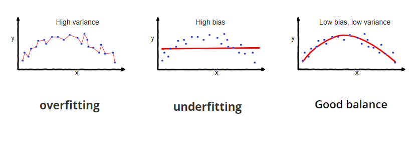
Bias and Variance What does that bias and variance actually mean? Let us understand this by an example below.

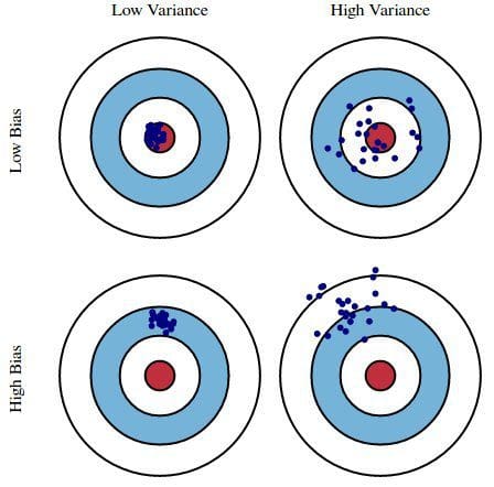
Let’s say we have model which is very accurate, therefore the error of our model will be low, meaning a low bias and low variance as shown in first figure. Similarly we can say that if the variance increases, the spread of our data point increases which results in less accurate prediction. And as the bias increases the error between our predicted value and the observed values increases. Now how this bias and variance is balanced to have a perfect model? Take a look at the image below and try to understand.

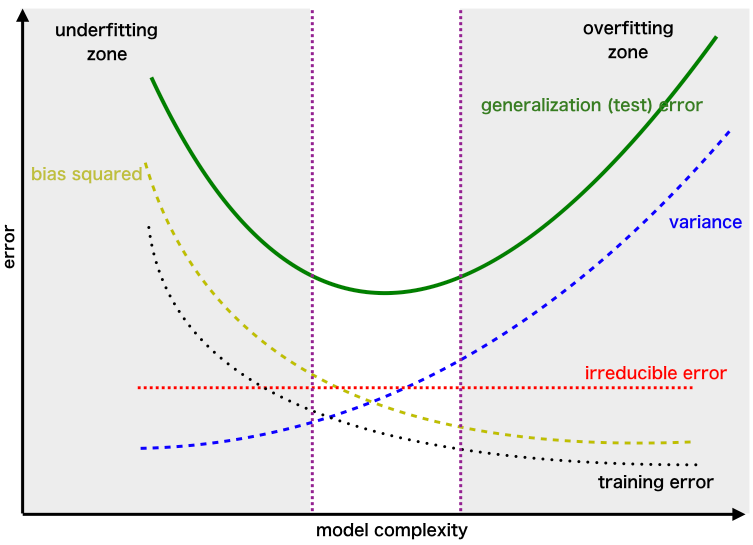
As we add more and more parameters to our model, its complexity increases, which results in increasing variance and decreasing bias, i.e., over fitting. So we need to find out one optimum point in our model where the decrease in bias is equal to increase in variance. In practice, there is no analytical way to find this point. So how to deal with high variance or high bias? To overcome under fitting or high bias, we can basically add new parameters to our model so that the model complexity increases, and thus reducing high bias.

Now, how can we overcome Overfitting for a regression model? Basically there are two methods to overcome overfitting,

• Reduce the model complexity
• Regularization

Here we would be discussing about model fitting and Regularization in detail and how to use it to make your model more generalized.

Over-fitting and Under-fitting in regression models

In above gif, the model tries to fit the best line to the trues values of the data set. Initially the model is so simple, like a linear line going across the data points. But, as the complexity of the model increases i..e. because of the higher terms being included into the model. The first case here is called under fit, the second being an optimum fit and last being an over fit.

Have a look at the following graphs, which explains the same in the pictorial below.

The trend in above graphs looks like a quadratic trend over independent variable X. A higher degree polynomial might have a very high accuracy on the train population but is expected to fail badly on test data set. In this post, we will briefly discuss various techniques to avoid over-fitting. And then focus on a special technique called Regularization.

Over fitting happens when model learns signal as well as noise in the training data and wouldn’t perform well on new data on which model wasn’t trained on. In the example below, you can see under fitting in first few steps and over fitting in last few.

Methods to avoid Over-fitting:

Following are the commonly used methodologies :

• Cross-Validation : Cross Validation in its simplest form is a one round validation, where we leave one sample as in-time validation and rest for training the model. But for keeping lower variance a higher fold cross validation is preferred.
• Early Stopping : Early stopping rules provide guidance as to how many iterations can be run before the learner begins to over-fit.
• Pruning : Pruning is used extensively while building CART models. It simply removes the nodes which add little predictive power for the problem in hand.
• Regularization : This is the technique we are going to discuss in more details. Simply put, it introduces a cost term for bringing in more features with the objective function. Hence, it tries to push the coefficients for many variables to zero and hence reduce cost term.

Now, there are few ways you can avoid over fitting your model on training data like cross-validation sampling, reducing number of features, pruning, regularization etc.

Regularization

Regularization helps to solve over fitting problem which implies model performing well on training data but performing poorly on validation (test) data. Regularization solves this problem by adding a penalty term to the objective function and control the model complexity using that penalty term.

Regularization is generally useful in the following situations: Large number of variables Low ratio of number observations to number of variables High Multi-Collinearity

Regularization basically adds the penalty as model complexity increases. Below is the equation of cost function Regularization parameter (lambda) penalizes all the parameters except intercept so that model generalizes the data and won’t over fit.

A simple linear regression is an equation to estimate y, given a bunch of x. The equation looks something as follows :

y = a1x1 + a2x2 + a3x3 + a4x4 ……. In the above equation, a1, a2, a3 … are the coefficients and x1, x2, x3 .. are the independent variables. Given a data containing x and y, we estimate a1, a2 , a3 …based on an objective function. For a linear regression the objective function is as follows :

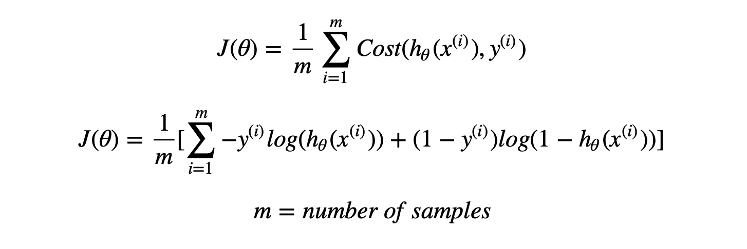
Now, this optimization might simply overfit the equation if x1 , x2 , x3 (independent variables ) are too many in numbers. Hence we introduce a new penalty term in our objective function to find the estimates of co-efficient. Following is the modification we make to the equation :

The new term in the equation is the sum of squares of the coefficients (except the bias term) multiplied by the parameter lambda. Lambda = 0 is a super over-fit scenario and Lambda = Infinity brings down the problem to just single mean estimation. Optimizing Lambda is the task we need to solve looking at the trade-off between the prediction accuracy of training sample and prediction accuracy of the hold out sample.

How can we choose the regularization parameter λ?

If we choose lambda = 0 then we get back to the usual OLS estimates. If lambda is chosen to be very large then it will lead to underfitting. Thus it is highly important to determine a desirable value of lambda.To tackle this issue, we plot the parameter estimates against different values of lambda and select the minimum value of λ after which the parameters tend to stabilize.

Ridge, Lasso and Elastic-Net Regression

Ridge, LASSO and Elastic net algorithms work on same principle. They all try to penalize the coefficients so that we can get the important variables (all in case of Ridge and few in case of LASSO). They shrink the beta coefficient towards zero for unimportant variables. These techniques are well being used when we have more numbers of predictors/features than observations. The only difference between these 3 techniques are the alpha value. If you look into the formula you can find the important of alpha.

Here lambda is the penalty coefficient and it’s free to take any allowed number while alpha is selected based on the model you want to try .

So if we take lambda = 0, it will become Ridge and lambda = 1 is LASSO and anything between 0–1 is Elastic net.

L1 Regularization and L2 Regularization

Ridge and Lasso regression are powerful techniques generally used for creating parsimonious models in presence of a ‘large’ number of features.

Though Ridge and Lasso might appear to work towards a common goal, the inherent properties and practical use cases differ substantially.

Ridge Regression:

• Performs L2 regularization, i.e. adds penalty equivalent to square of the magnitude of coefficients
• Minimization objective = LS Obj + α * (sum of square of coefficients) Lasso Regression:
• Performs L1 regularization, i.e. adds penalty equivalent to absolute value of the magnitude of coefficients
• Minimization objective = LS Obj + α * (sum of absolute value of coefficients)

In order to create less complex (parsimonious) model when you have a large number of features in your dataset, some of the Regularization techniques used to address over-fitting and feature selection are:

A regression model that uses L1 regularization technique is called Lasso Regression and model which uses L2 is called Ridge Regression.

Elastic Net regression is preferred over both ridge and lasso regression when one is dealing with highly correlated independent variables. It is a combination of both L1 and L2 regularization.

Why do we use Regularization?

Traditional methods like cross-validation, step wise regression to handle over fitting and perform feature selection work well with a small set of features but these techniques are a great alternative when we are dealing with a large set of features.

Gradient Descent Approach

There is also another technique other than regularization which is also used widely to optimize the model and avoid the chances of over fitting in your model, which is called Gradient Descent. Gradient descent is a technique we can use to find the minimum of arbitrarily complex error functions.

In gradient descent we pick a random set of weights for our algorithm and iteratively adjust those weights in the direction of the gradient of the error with respect to each weight. As we iterate, the gradient approaches zero and we approach the minimum error.

In machine learning we often use gradient descent with our error function to find the weights that give the lowest errors.

Here is an example with a very simple function.

The gradient of this function is given by the following equation. We choose an random initial value for x and a learning rate of 0.1 and then start descent. On each iteration our x value is decreasing and the gradient (2x) is converging towards 0.

The learning rate is a what is know as a hyper-parameter. If the learning rate is too small then convergence may take a very long time. If the learning rate is too large then convergence may never happen because our iterations bounce from one side of the minimum to the other. Choosing a suitable value for hyper-parameters is an art so try different values and plot the results until you find suitable values.

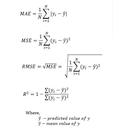
Performance Criteria

Mean Squared Error

The root mean squared error in a linear regression problem is given by the equation 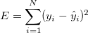which is the sum of squared differences between the actual value and the predicted value for each of the rows in the dataset (index iterated over i).

R-Squared

R-squared is a statistical measure of how close the data are to the fitted regression line. It is also known as the coefficient of determination, or the coefficient of multiple determination for multiple regression. R-sqaure is given by the following formula 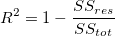The idea is to minimize so as to keep the value of as close as possible to 1. The calculation essentially gives us a numeric value as to how good is our regression line, as compared to the average value.

Adjusted R-Squared

The value of is considered to be better as it gets closer to 1, but there’s a catch to this statement. The value can be artifically inflated by simply adding more variables. This is a problem because the complexity of the model would increase due to this and would result in overfitting. The formulae for Adjusted R-squared is mathematically given as: 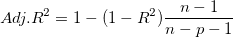where p is the number of regressors and n is the sample size. Adjusted R-squared has a penalizing factor that reduces it’s value when a non-significant variable is added to the model.

p-value based backward elimination can be useful in removing non-significant variables that we might have added in our model initially.

---

Want to support this project? Contribute..

References

1. https://towardsdatascience.com/introduction-to-machine-learning-algorithms-linear-regression-14c4e325882a
2. https://machinelearningmastery.com/linear-regression-for-machine-learning/
3. https://ml-cheatsheet.readthedocs.io/en/latest/linear_regression.html
4. https://machinelearningmastery.com/implement-simple-linear-regression-scratch-python/
5. https://medium.com/analytics-vidhya/linear-regression-in-python-from-scratch-24db98184276
6. https://scikit-learn.org/stable/auto_examples/linear_model/plot_ols.html
7. https://scikit-learn.org/stable/modules/generated/sklearn.compose.TransformedTargetRegressor.html