Introduction

A times series is a set of data recorded at regular times. For example, you might record the outdoor temperature at noon every day for a year.

The movement of the data over time may be due to many independent factors.

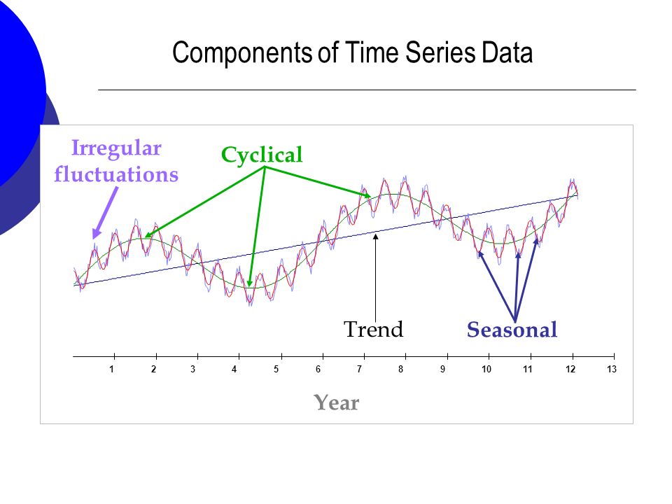
Long term trend: the overall movement or general direction of the data, ignoring any short term effects such as cyclical or seasonal variations. For example, the enrollment trend at a particular university may be a steady climb on average over the past 100 years. This trend may be present despite having a few years of loss or stagnant enrollment followed by years of rapid growth. Cyclical Movements: Relatively long term patterns of oscillation in the data. These cycles may take many years to play out. There is a various cycles in business economics, some taking 6 years, others taking half a century or more. Seasonal Variation: Predictable patterns of ups and downs that occur within a single year and repeat year after year. Temperatures typically show seasonal variation, dropping in the Fall and Winter and rising again in the Spring and Summer. Noise: Every set of data has noise. These are random fluctuations or variations due to uncontrolled factors.

Putting the Factors Together

Each factor has an associated data series:

• Trend factor: Tt
• Cyclic factor: Ct
• Seasonal factor: St
• Noise factor: Nt Finally, the original data series, Yt, consists of the product of the individual factors.

Yt = Tt × Ct × St × Nt

Often only one of the oscillating factors, Ct or St, is needed.

Forecasting

The idea behind forecasting is to predict future values of data based on what happened before. It’s not a perfect science, because there are typically many factors outside of our control which could affect the future values substantially. The further into the future you want to forecast, the less certain you can be of your prediction.

Just look at weather reporting! Figuring out if it will rain tomorrow is not too difficult, but it’s virtually impossible to predict if it will rain exactly a month from now.

Basically, the theory behind a forecast is as follows.

1. Smooth out all of the cyclical, seasonal, and noise components so that only the overall trend remains.
2. Find an appropriate regression model for the trend. Simple linear regression often does the trick nicely.
3. Estimate the cyclical and seasonal variations of the original data.
4. Factor the cyclical and seasonal variations back into the regression model.
5. Obtain estimates of error (confidence intervals). The larger the noise factor, the less certain the forecasted data will be.

Key Terms

There are a few key terms that are commonly encountered when working with Time Series, these are inclusive of but not exclusively described in the following list:

Trend: A time series is supposed to have an upward or downward trend if the plot shows a constant slope when plotted. It is noteworthy that for a pattern to be a trend, it needs to be consistent through the series. If we start getting upwards and downwards trend in the same plot, then it could be an indication of cyclical behavior.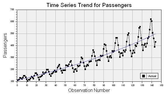

Sesonality: If a TS has a regular repeating pattern based on the calendar or clock, then we call it to have seasonality. Soemtimes there can be different amount of seasonal variation across years, and in such cases it is ideal to take the log of values in order to get a better idea about seasonality. It is noteworthy that Annual Data would rarely have a seasonal component.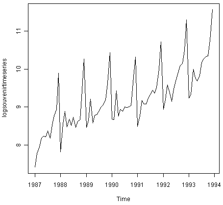

Cyclical TS: Cyclical patterns are irregular based on calendar or clock. In these cases there are trends in the Time Series that are of irregular lengths, like business data, there can be revenue gain or loss due to a bad product but how long the upward or downward trend would last, is unknown beforehand. Often, when a plot shows cyclical behavior, it would be a combination of big and small cycles. Also, these are very difficult to model because there is no specific pattern and we do not know what would happen next.

Autocorrelation/Serial Correlation: The dependence on the past in case of a univariate time series is called autocorrelation.

Types of Time Series

The two major types of time series are as follows:

Most of the theory that has been developed was developed for stationary time series.

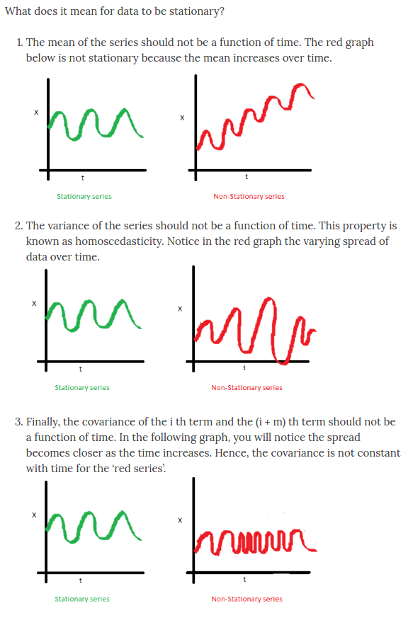
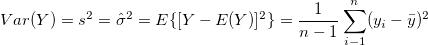
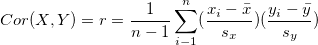
1. Stationary: Such time series have constant mean and reasonably constant variance through time. eg. annual rainfall
2. Non-Stationary: If we have a non-stationary time series then there are additional patterns in our series, like Trends, Seasonality or Cycles. These do not necessarily have a constant mean variance through time.

a. **Univariate Time Series**: We usually use regression technique to model non-stationary time series and we also have to consider the time series aspects (like autocorrelation i.e. dependence on the past and differencing, i.e. the technique used in TS to try and get rid of autocorrelation). **If we have a Time Series with trend, seasonality and non-constant variance, then it is best to log the data which would then allow us to stabilize the variance, hence the name 'Variance Stablizing Transformation' This allows us to fit our data in additive models, making it a very useful technique.** 

b. **Multivariate Time Series**: Many variables measured through time, typically measured on the same time points. In some other cases, they may be measured on different time points but within an year. Such data would need to be analyzed using multiple regression models. We might also want to fit the time variable in the model (after transformations maybe) but this could allow us to determince whether there was any **trend** in the response and capture it. If you do not find any trend in the data, then the time variable can be chucked out but **modelling the data without checking for the time variable would be a horrible idea**.

More observations is often a good thing because it allows greater degrees of freedom. (Clarification needed, will read a few paper to better this concept)

1. Panel Data/Logitudinal Data: Panel data is a combination of cross-sectional data and time series. There can be two kinds of time logging for panel data, implicit and explicit. In econometrics and finance studies, the time is implicitly marked which in areas like medical studies explicit marking of time is done on Panel data. The idea is to take a cross-sectional measurements at some point in time and then repeat the measurements again and again to form a time series.

2. Continuous Time Models: In this kind of data, we have a Point(Time component) process and a Stochastic (Random) process. For instance, the number of people arriving at a particular restaurant is an example of this where the groups of people ae arriving at certain points in time(point process) and the size of the group is random (stochastic process).

NOTE: No matter what a time series data is about, on the axis (while modeling) we always use a sequence of numbers starting from 1, up to the total number of observations. This allows us to focus on the sequence of measurements because we already know the frequency the time interval between any two observations.

Features of Time Series

A few key features to remember when modelling time series are as follows:

1. Past will affect the future but the future cannot affect the past
2. There will rarely be any independence between observations, temperature, economics and all other major fields have dependence on the past in case of Time Series data
3. The pattern is often exploited to predict and build better models
4. Stationary techniques can be used to model non-stationary time series, and also to remove trends, seasonality, and sometimes even cycles.
5. We can also try to decompose time series into various components, model each one of them separately and then forecast each of the components and then combine again.
6. we also use Moving Averages (also known as filtering or smoothing) because it tries to remove the seasonal component of time series.
7. We would often also need to transform the data before it can be used. The most common time we need to do transformations in Time Series is when we have an increasing seasonal variation because that represents a multiplicative model, which can be hard to explain.

Autocorrelation

The general concept of dependence on the past is called autocorrelation in statistics. If we are going to use regression models for mdoeling non-stationary data, we need to ensure that they satisfy the underlying assumptions necessary for regression models, i.e. normally distributed, zero mean, constant variance in the residual plot.

Variance, Covariance and Correlation

Variance

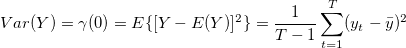
The population variance denoted by is calculated using the sample variance. For any given sample Y, it’s variance is calculated as follows:

Note: Variance is a special case of covariance, it just means how the sample of observations varies with itself.

Covariance

It tells us how two varaibles vary with each other. Simply put, are the large values of X related to large values in Y or are the large values in X related to small values in Y? It is calculated as follows:

Correlation

Standardized covariance is called correlation, therefore it always lies between -1 and 1. It is represented as

where represented the standard deviation for x and represents the standard deviation for y.

Autocorrelation takes place for univariate time series.

Sample Autovariance

Covariance is with respect to itself in this case, for the past values that have occurred in time and is represented as follows.

Sample Autocovariance

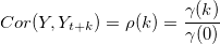
In a univariate time series, the covariance between two observations k time periods apart (lag k), is given by

Sample Autocorrelation

Standardized autocovariance is equal to sample autocorrelation (k time periods apart) which is denoted by and is given as follows:

Detecting Autocorrelation

There are two types of autocorrelation that we look for:

1. Positive Autocorrelation: Clustering in Residuals
2. Negative Autocorrelation: Oscillations in Residuals (this is rare)

The following methods are used for detecting autocorrelation:

Use the tests

Durbin Watson Test (usually used in Econometrics)

Plot of Current vs Lagged residuals

Runs (Geary) Test

Chi-Squared Test of Independence of Residuals

Autocorrelation Function (ACF)

This function does the tests for all possible lags and plots them at the same time as well. It is very time efficient for this reason.

Time Series Regression

There are certain key points, that need to be considered when we do, Time Series Regression. They are as follows:

1. Check if time ordered residuals are independent
2. White Noise: Time Series of independent residuals (i.e. independent and identically distributed (iid), normal with 0 mean and constant variance ) It is given by
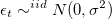
3. When doing regression models of nonstationary time series, check for autocorrelation in the residual series, because a pattern in the residual series is equivalent to pattern in the data not captured by our model.

Seasonality

Smoothing or Filtering

Often the smoothing or filtering is done before the data is delivered and this can be bad thing because we don’t know how seasonality was removed and also because we can only predict deseasonal values.

STL (Seasonal Trend Lowess Analysis

We can also do an STL analysis which would give us the seasonality, trend and remainder plots for any time series.

NOTE: If you find that the range of the seasonality plot is more or less the same as the range of the remained plot, then there isn’t much seasonality. The STL is designed to look for seasonality so it will always give you a seasonality plot and it’ll be for the person reading to determine whether there is actual seasonlity or not.

Moving Averages

Both can be used to remove seasonality

Want to support this project? Contribute..